DeformSolid / Computational geometry

Model the solid.
Follow the deformation.

Model and edit solids after nonlinear deformation.FE-aligned boundaries made sampled geometry 105× more accurate at the finest tested resolution.

3D BooleanFinite-element geometryC++

Explore the geometry ↓Read the code ↗

Actual generated reference four-hole solid, nonlinear deformation, spatial Boolean result, and enlarged cut detail — One four-hole component. A nonlinear map. Actual three-dimensional material removal.

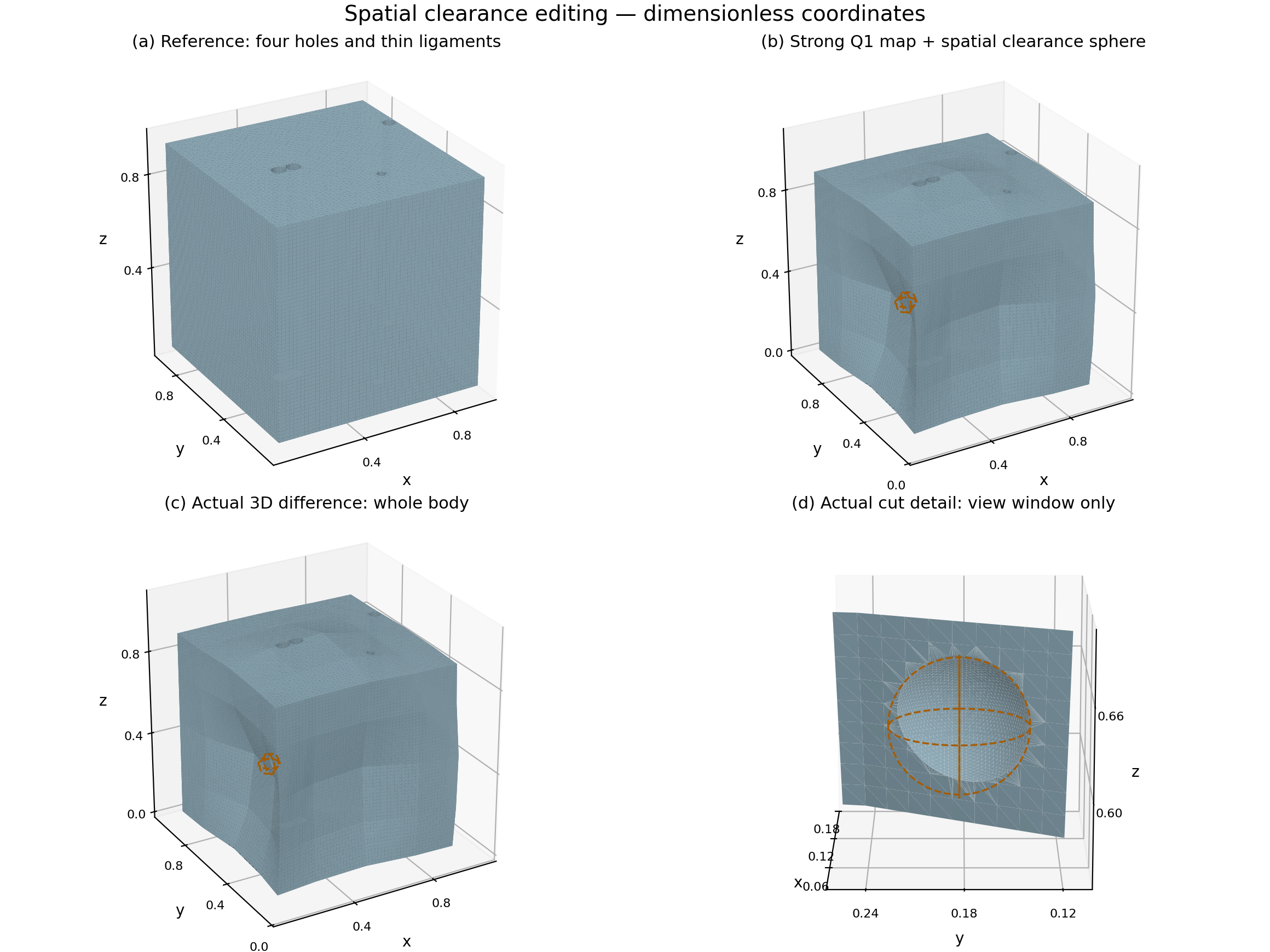
01 / Interactive geometry

One model. Five ways to inspect it.

Rotate the actual mesh, compare operations, and move inside the cut. These are the generated geometry outputs.

B / Deform, then cutLoading geometry…

Drag to rotate · Scroll to zoom · Arrow keys supported

Reveal interior Download OBJ ↓

Rotate the meshes, reveal their interiors, and download double-precision OBJ geometry.

02 / Operations under deformation

The cutting tool has a coordinate system.

Cutting in reference space and cutting in the deformed scene answer different geometric questions. Transporting the tool connects them.

Cut, then deform

Remove the reference-space sphere B₀, then map the remaining solid.

Φ(Ω₀ ∖ B₀)

Deform, then cut

Subtract the independently specified spatial sphere B₁ from the deformed body.

Φ(Ω₀) ∖ B₁

Transport the tool

Map B₀ with the body, then execute a 3D Boolean in deformed space.

Φ(Ω₀) ∖ Φ(B₀)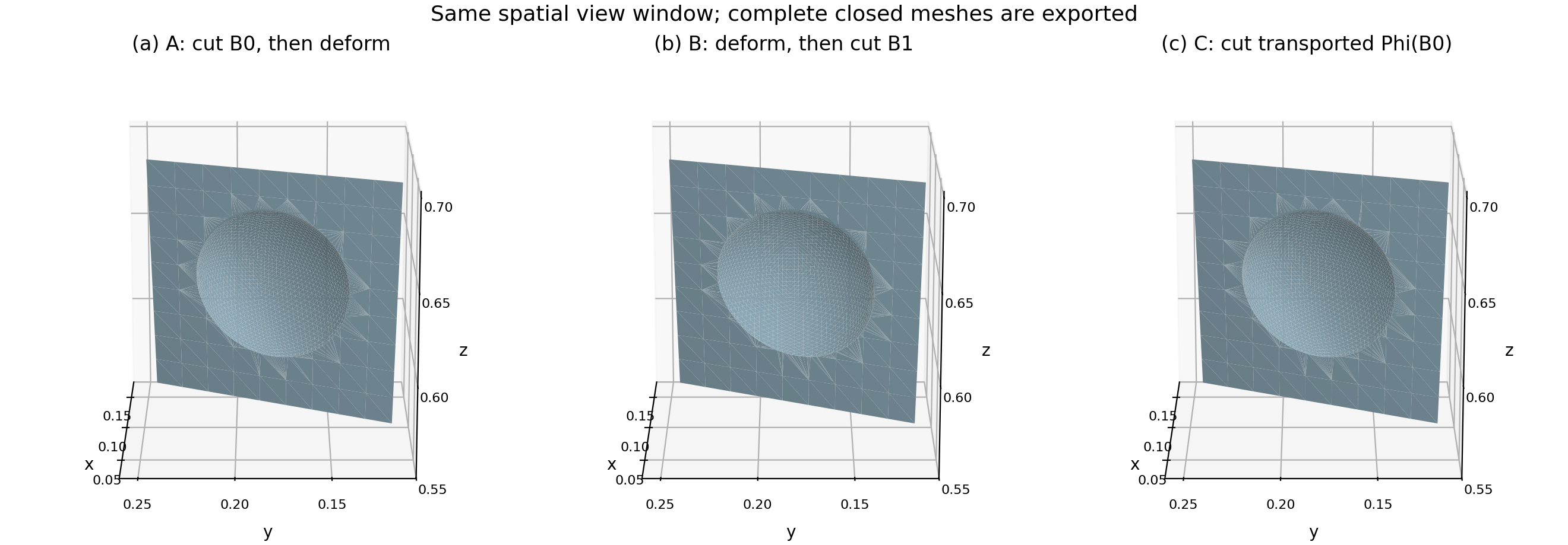

Matching local three-dimensional views of cut-first, spatial-cut, and transported-tool Boolean outputs — A and C describe the same continuous target. Their sampled surface discrepancy decreases from 2.73 × 10⁻⁴ to 6.56 × 10⁻⁵ on refinement. B uses the established independently placed spatial sphere.

Tool placement

B₀: center (0.0525, 0.18, 0.62), radius 0.045. B₁: center (0.09942443490438002, 0.183131631211526, 0.6264289927536667), radius 0.045. The transported Φ(B₀) is generally not a sphere. Coordinates and volumes are dimensionless.

03 / Cross-section inspection

Look through the shape.

Compare closed contours at three fixed heights. Every displayed section has one material component and four holes.

A · Cut firstB · Cut afterC · Transported tool

Fine-mesh contours are shown in a shared coordinate frame. Independent inverse-field sections and local comparisons are in the section figure ↗.

04 / FE-aware accuracy

Follow the element boundaries.

A deformed solid is reconstructed from a finite-element map. Its slope changes across element interfaces; edges crossing those interfaces can carry extra geometric error into the final Boolean output.

105.48×

Smaller finest-level sampled geometric error with FE-aligned boundary reconstruction.

0.975 → 1.954

Observed convergence orders: without versus with FE alignment.

+3.75%

Input triangle count at the finest resolution.

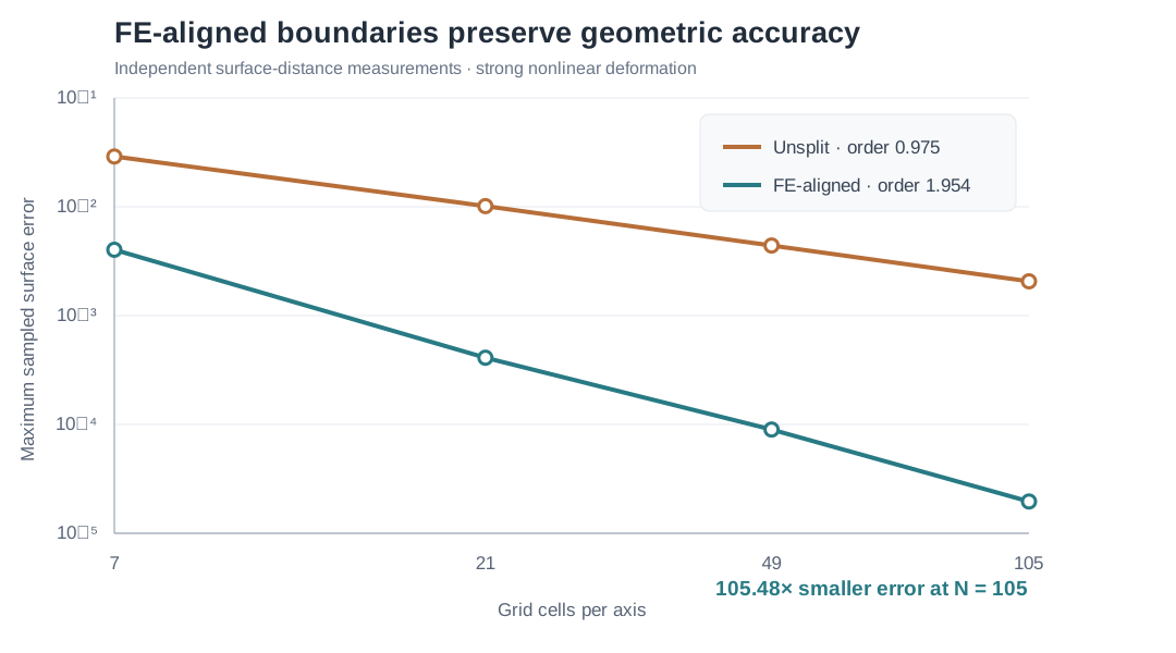
Measured maximum sampled surface errors at four resolutions: the unsplit boundary converges near first order; the FE-aligned boundary approaches second order. — Measured sampled distances, same strong deformation and independent reference points. No continuous error or topology certificate is claimed. Download plotted values ↓

At the finest resolution, sampled maximum error decreased from 2.066 × 10⁻³ to 1.958 × 10⁻⁵. Four follow-up 3D Boolean outputs passed mesh checks and kept the expected four-hole sections. A separate standalone matched-input splitter exposed seam gaps near 10⁻¹³; the supported result is for the complete FE-aligned construction.

05 / High-performance compute

Geometry queries, built to batch.

A native C++ evaluator performs the Q1 map, damped Newton inversion, and analytic CSG field evaluation in double precision. No per-query Python calls.

7.2×

Native CPU speedup
at 2048² cells

4.9M/s

Dense query throughput
single-thread C++

9.52× 10⁻¹⁵

Maximum field difference
against Python

Batch queries

Caller-owned buffers and a stable structure-of-arrays C ABI.

Native C++

Q1 mapping → Newton inverse → analytic CSG → per-query status.

NumPy integration

Contiguous arrays connect native batch evaluation to Python geometry workflows.

Strong four-hole solid · measured CPU medians
Grid cells	C++	Python	Ratio
512²	0.0531 s	0.4091 s	7.71×
1024²	0.2146 s	1.5482 s	7.21×
2048²	0.8514 s	6.1203 s	7.19×

One warmup and five measured runs per method/grid, single-thread CPU. Native compute excludes allocation and interop; Python uses the existing chunked reference path. These are measured implementation ratios. Download timings ↓

06 / Geometric consistency

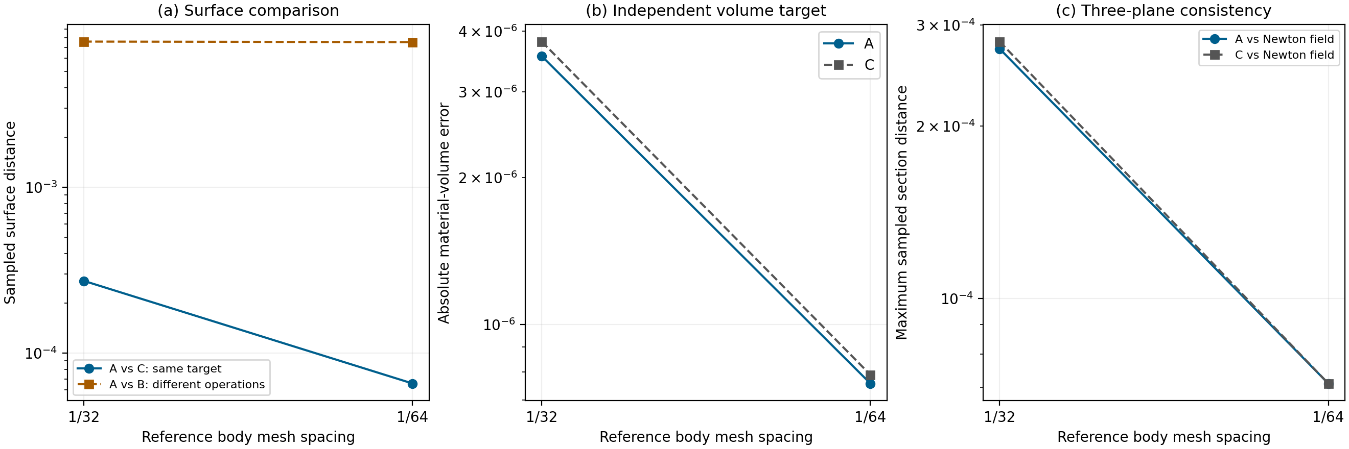
Keep the features. Measure the error.

Mesh validity, closed contours, independent volume integration, and refinement connect the 3D result to its implicit definition.

4 holes

Retained in all six comparison solids and all eighteen inspected mesh sections.

6.56 × 10⁻⁵

Fine A/C sampled surface distance for the transported-tool equivalence.

7.89 × 10⁻⁷

Fine transported-tool result's absolute volume error against independent Q1 integration.

Independent implicit-field checks covered twelve saved 3D Boolean meshes (49,636 point–mesh comparisons). All 4,214 definite label differences were within 1.892 × 10⁻⁴ of the mesh surface; 120 representative independent checks passed. They are sampled geometric differences near approximated boundaries, not exact label identity. Exp09 validation summary ↓

Measured surface distance, volume error, and section error at two mesh refinement levels — Two established refinement levels. Distances are sampled geometric comparisons; the raw measurements are available below.

Build / Explore / Extend

Open the model. Follow the code.

The current release brings together the modeling application, the native C++ numerical engine, inspectable meshes, and measured results.

Code ↗Download a mesh ↓

Surface comparison Volume comparison Section comparison Mesh measurements

Model the solid.Follow the deformation.